Learning to learn – What to look for in the evaluation of classification

Applying some machine learning algorithm to classify some data is made easy these days. There is a large amount of programming libraries, applications and online services available on the market. But how do we know whether the algorithm works? Or which of the methods to chose from is the best for our task? This post will give a very short introduction to the four most relevant issues in the evaluation of classification results. None of these points is restricted to a specific machine learning algorithm. In fact, none of them requires any understanding of the used classification method at all.

1. Good machine learning requires good data
The first and most obvious point is, that machine learning requires training data. Training data consists of a number of data items with associated labels assigned by humans. For example, we could train on a set of e-mails which have been labeled as spam or non-spam by the person receiving them. In order for a learning algorithm to learn something useful, a few conditions should be met by the training data. First, there should be enough data. Learning from only 100 e-mails will not work, as there are many types of spam mails. Second, the data should be as clean as possible. If half of the spam-labels are wrong, there is no way how an algorithm can learn what real spam is. And finally, the data should also be as close as possible to the real data that you want to classify later. Training a spam-recognition system on English and then apply it to German will probably not work well.

2. Don’t evaluate on your training data
After the machine learning algorithm has learned to distinguish the classes on the training data, it is ready to be applied to new data. Based on what it has learned from the training data, the algorithm will assign a class to each new data item. A common beginner’s mistake is to apply the algorithm to the training data again. This will lead to very good results, but these results are misleading. Imagine that the “learning algorithm” is just memorizing complete e-mails. If the exact same e-mail is shown to the algorithm again, it will confidently assign the correct class. 100% of training set e-mails will be correct! But even changing one word will cause the algorithm to fail, so it is no use to us in reality. Of course real learning algorithms are more complex, but the issue is the same. It is very easy to be confident about what you already have seen. The hard part is to deal with new stuff. So in order to have a reliable evaluation, the algorithm should be trained on one data set and applied to another totally separate set.

3. Evaluate on data that is close to the data you want to classify later
As we have just discussed, we need to evaluate on data that is different from the training data. But, just like the training data, the evaluation data should be as close as possible to the real data that you want to classify later. If you want to classify German, it doesn’t help you to know that the spam-classifier works very well on English. A common procedure for a good evaluation is to create one data set with labeled data, and then split it up into training and test data (e.g., 80% training data, 20% test data). No item is allowed to be in both sets at the same time. Another common technique is called k-fold cross-validation. This method splits the data into k (often 10) folds and does k train-test runs. In each run, one of the folds is used as test data and the other folds are used as training data. The folds do not change between runs, so in the end every item in the data has been assigned a label, but at that point this item was not in the training set, so point 2 is not violated. For both technique it is worth thinking about whether to randomly shuffle the folds or to enforce a similar label-distribution in all the folds in order to avoid artificial inflation of the results.

4. Chose the right evaluation metric for your problem
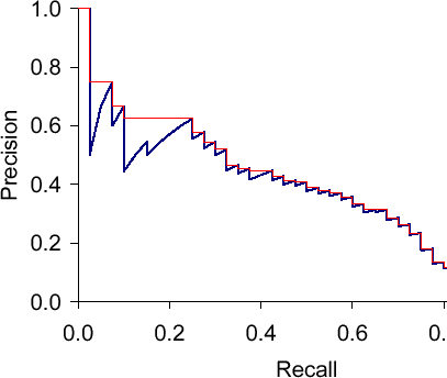
After the machine learning system has assigned a class to every data item, we compare the assigned labels to the real labels. The larger the percentage of correct labels, the better the system. There are many ways of comparing the labels depending on the nature of the labels and their distribution. The simplest measure, called accuracy, is to count the number of correct assignments, e.g., how many real spam-mails have been classified as spam by the system and how many non-spam-mails have been classified as non-spam. But accuracy is not a good measure in some cases. Let’s assume that 90% of mails are non-spam. If a system always assigns the label non-spam, it will be 90% accurate – but not useful at all. The same thing happens with many classes if some are much bigger than the others. Accuracy is also not a good choice when labels are on a scale. In this case confusing 1 and 5 is much more serious than confusing 1 and 2 and accuracy does not reflect this. There are alternative metrics for such scenarios that should be used.

I will stop here, although there is more much to be said. I encourage everybody to investigate the topic in more detail. Good evaluation is at least as important as good machine learning algorithms. If evaluation numbers do not reflect the expected real performance of a system, how can they be the basis of any decision?


This post has first appeared at 5analytics.com

Precision, Recall and F-measure

In the last post we discussed accuracy, a straightforward method of calculating the performance of a classification system. Using accuracy is fine when the classes are of equal size, but this is often not the case in real world tasks. In such cases the very large number of true negatives outweighs the number of true positives in the evaluation so that accuracy will always be artificially high.

Luckily there are performance measures that ignore the number of true negatives. Two frequently used measures are precision and recall. Precision P indicates how many of the items that we have identified as positives are really positives. In other words, how precise have we been in our identification. How many of those that we think are X, really are X. Formally, this means that we divide the number of true positives by the number of all identified positives (true and false):
P = TP/(TP+FP)

Recall R indicates how many of the real positives we have found. So from all of the positive items that are there, how many did we manage to identify. In other words, how exhaustive we were. Formally, this means that we divide the number of true positives by the number of all existing positives (true positives and false negatives):
R = TP/(TP+FN)

For our example from the last post, precision and recall are as follows:
P = 1/(1+3) = 1/4 = 0.25
R = 1/(1+2) = 1/3 = 0.33

It is easy to get a recall of 100%. We just say for everything that it is a positive. But as this will probably not the case (or else we have a really easy dataset to classify!), this approach will give us a really low precision. On the other hand, we can usually get a high precision if we only classify as positive one single item that we are really, really sure about. But if we do that, recall will be low, as there will be more than one item in the dataset to be classified (or else it is not a very meaningful set).

So recall and precision are in a sort of balance. The F1 score or F1 measure is a way of putting the two of them together to produce one single number. Formally it calculates the harmonic mean of the two numbers and weights the two of them with the same importance (there are other variants that put more importance on one of them):
F_1 = (2 \cdot P \cdot R)/(P + R)

Using the values for precision and recall for our example, F1 is:
F_1 = (2 \cdot 0.25 \cdot 0.33)/(0.25 + 0.33) = 0.165 / 0.58 = 0.28

Intuitively, F1 is between the two values of precision and recall, but closer to the lower of the two. In other words, it penalizes if we concentrate only on one of the values and rewards systems where precision and recall are closer together.

Link for a second explanation: Explanation from an Information Retrieval perspective

Accuracy

We are still trying to figure out how good our system for determining whether e-mails are spam or not is. In the last post we ended up with a confusion matrix like this:

Actual label
Spam NonSpam
Predicted label Spam 1 (true positives, TP) 3 (false positives, FP)
NonSpam 2 (false negatives, FN) 4 (true negatives, TN)

Now we want to calculate numbers from this table to describe the performance of our system. One easy way of doing this is to use accuracy A. Accuracy basically describes which percentage of decisions we got right. So we would take the diagonal entries in the matrix (the true positives and true negatives) and divide by the total number of entries. Formally:
A = (TP+TN)/(TP+TN+FP+FN)

In our example the accuracy is:
A = (1+4)/(1+4+2+3) = 5/10 = 0.5

Using accuracy is fine in examples like the above when both classes occur more or less with the same frequency. But frequently the number of true negatives is larger than the number of true positives by many orders of magnitudes. So let’s assume 994 for true negatives and when we calculate accuracy again, we get this:
A = (1+994)/(1+994+2+3) = 995/1000 = 0.995

It doesn’t really matter if we correctly identify any spam mails. Even if we always say NonSpam, so we get zero Spam-Mails right, we still get more nearly the same accuracy as above. So accuracy is not a good indicator of performance for our system in this situation. In the next post we will look at other measures we can use instead.

Link for a second explanation: Explanation from an Information Retrieval perspective

Confusion matrix

Let’s say we want to analyze e-mails to determine whether they are spam or not. We have a set of mails and for each of them we have a label that says either "Spam" or "NotSpam" (for example we could get these labels from users who mark mails as spam). On this set of documents (the training data) we can train a machine learning system which given an e-mail can predict the label. So now we want to know how the system that we have trained is performing, whether it really recognizes spam or not.

So how can we find out? We take another set of mails that have been marked as "Spam" or "NotSpam" (the test data), apply our machine learning system and get predicted labels for these documents. So we end up with a list like this:

Actual label Predicted label
Mail 1 Spam NonSpam
Mail 2 NonSpam NonSpam
Mail 3 NonSpam NonSpam
Mail 4 Spam Spam
Mail 5 NonSpam NonSpam
Mail 6 NonSpam NonSpam
Mail 7 Spam NonSpam
Mail 8 NonSpam Spam
Mail 9 NonSpam Spam
Mail 10 NonSpam Spam

We can now compare the predicted labels from our system to the actual labels to find out how many of them we got right. When we have two classes, there are four possible outcomes for the comparison of a predicted label and an actual label. We could have predicted "Spam" and the actual label is also "Spam". Or we predicted "NonSpam" and the label is actually "NonSpam". In both of these cases we were right, so these are the true predictions. But, we could also have predicted "Spam" when the actual label is "NonSpam". Or "NonSpam" when we should have predicted "Spam". So these are the false predictions, the cases where we have been wrong. Let’s assume that we are interested in how well we can predict "Spam". Every mail for which we have predicted the class "Spam" is a positive prediction, a prediction for the class we are interested in. Every mail where we have predicted "NonSpam" is a negative prediction, a prediction of not the class we are interested in. So we can summarize the possible outcomes and their names in this table:

Actual label
Spam NonSpam
Predicted label Spam true positives (TP) false positives (FP)
NonSpam false negatives (FN) true negatives (TN)

The true positives are the mails where we have predicted "Spam", the class we are interested in, so it is a positive prediction, and the actual label was also "Spam", so the prediction was true. The false positives are the mails where we have predicted "Spam" (a positive prediction), but the actual label is "NonSpam", so the prediction is false. Correspondingly the false negatives, the mails we should have labeled as "Spam" but didn’t. And the true negatives that we correctly recognized as "NonSpam". This matrix is called a confusion matrix.

Let’s create the confusion matrix for the table with the ten mails that we classified above. Mail 1 is "Spam", but we predicted "NonSpam", so this is a false negative. Mail 2 is "NonSpam" and we predicted "NonSpam", so this is a true negative. And so on. We end up with this table:

Actual label
Spam NonSpam
Predicted label Spam 1 3
NonSpam 2 4

In the next post we will take a loo at how we can calculate performance measures from this table.

Link for a second explanation: Explanation from an Information Retrieval perspective

Precision-Recall-Curves and Mean Average Precision

Precision-recall curves are often used to evaluate ranked results of an information retrieval system (e.g., a search engine). The principle is easy, for every search result, check the precision and recall you have until now (precision/recall at k). If you plot this in a graph with recall on the x-axis and precision on the y-axis, you end up with something like this (blue line):

The essential shape is always the same. Why? Let’s say we have looked at k results which corresponds to a point with a precision and a recall value. What can happen when we go to result k+1? The result can be correct, then recall will increase and precision as well – the curve goes up and right. Or it can go wrong, then recall stays the same and precision drops – the curve goes straight down.

The red line is the interpolated precision, meaning we define precision at some arbitrary level to be the maximum precision reached at any later recall level. Essentially, we flatten the "teeth" of the curve. The difference can be pretty big (see in the plot at recall around 0.2), we can even "skip" a tooth.

What would the curve look like for a perfect system? Meaning a system that only returns correct results? It would be 1.0 for every recall level. A system that never returns a correct result? 0 for every recall level.

What should the value be for precision at recall 0? If we interpolate, the answer is clear: the highest precision value at some later recall level. This does not have to be 1.0 – it could happen that the first result is wrong, the second correct, then we have P=0.5 at k=2 and it might only drop from there.


Sancho McCann. It’s a bird… it’s a plane… it depends on your classifier threshold. 2011.
Christopher D. Manning, Prabhakar Raghavan and Hinrich Schütze. Introduction to Information Retrieval. Cambridge University Press, 2008. (Chapter 8)